Taiwan Election Data
 [1] "District"        "Sex"             "Age"             "Edu"
 [5] "Arear"           "Career"          "Career8"         "Ethnic"
 [9] "Party"           "PartyID"         "Tondu"           "Tondu3"
[13] "nI2"             "votetsai"        "green"           "votetsai_nm"
[17] "votetsai_all"    "Independence"    "Unification"     "sq"
[21] "Taiwanese"       "edu"             "female"          "whitecollar"
[25] "lowincome"       "income"          "income_nm"       "age"
[29] "KMT"             "DPP"             "npp"             "noparty"
[33] "pfp"             "South"           "north"           "Minnan_father"
[37] "Mainland_father" "Econ_worse"      "Inequality"      "inequality5"
[41] "econworse5"      "Govt_for_public" "pubwelf5"        "Govt_dont_care"
[45] "highincome"      "votekmt"         "votekmt_nm"      "Blue"
[49] "Green"           "No_Party"        "voteblue"        "voteblue_nm"
[53] "votedpp_1"       "votekmt_1"
Call:
glm(formula = votetsai ~ female, family = binomial, data = TEDS_2016)

Deviance Residuals:
    Min       1Q   Median       3Q      Max
-1.4180  -1.3889   0.9546   0.9797   0.9797

Coefficients:
            Estimate Std. Error z value Pr(>|z|)
(Intercept)  0.54971    0.08245   6.667 2.61e-11 ***
female      -0.06517    0.11644  -0.560    0.576
---
Signif. codes:  0 '***' 0.001 '**' 0.01 '*' 0.05 '.' 0.1 ' ' 1

(Dispersion parameter for binomial family taken to be 1)

    Null deviance: 1666.5  on 1260  degrees of freedom
Residual deviance: 1666.2  on 1259  degrees of freedom
  (429 observations deleted due to missingness)
AIC: 1670.2

Number of Fisher Scoring iterations: 4
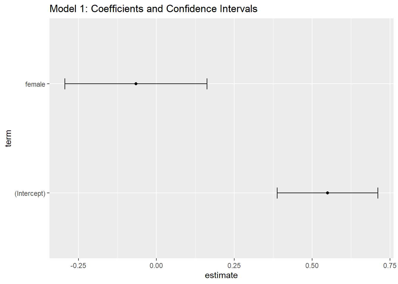
Interpreting the first logistic regression model
Based on the output of the logistic regression model, the coefficient for the female variable is -0.06517, and the p-value is 0.576. Since the p-value is greater than the standard significance level of 0.05, we fail to reject the null hypothesis, and there is no evidence to suggest that female voters are more likely to vote for President Tsai than male voters in this model.
The intercept of the model is 0.54971, which represents the log-odds of votetsai (voting for Tsai Ing-wen) for the reference group (male voters) in this case. The negative coefficient for the female variable (-0.06517) indicates that the log-odds of votetsai for female voters are slightly lower than for male voters, but this difference is not statistically significant.
It is essential to note that this model only includes the female predictor variable. Adding more variables (e.g., party ID, demographics, or issue-specific variables) may improve the model and provide more insights into factors affecting voting for President Tsai, which is what the next section will attempt to do.
Call:
glm(formula = votetsai ~ female + KMT + DPP + age + edu + income,
    family = binomial, data = TEDS_2016)

Deviance Residuals:
    Min       1Q   Median       3Q      Max
-2.7360  -0.3673   0.2408   0.2946   2.5408

Coefficients:
             Estimate Std. Error z value Pr(>|z|)
(Intercept)  1.618640   0.592084   2.734  0.00626 **
female       0.047406   0.177403   0.267  0.78930
KMT         -3.156273   0.250360 -12.607  < 2e-16 ***
DPP          2.888943   0.267968  10.781  < 2e-16 ***
age         -0.011808   0.007164  -1.648  0.09931 .
edu         -0.184604   0.083102  -2.221  0.02632 *
income       0.013727   0.034382   0.399  0.68971
---
Signif. codes:  0 '***' 0.001 '**' 0.01 '*' 0.05 '.' 0.1 ' ' 1

(Dispersion parameter for binomial family taken to be 1)

    Null deviance: 1661.76  on 1256  degrees of freedom
Residual deviance:  836.15  on 1250  degrees of freedom
  (433 observations deleted due to missingness)
AIC: 850.15

Number of Fisher Scoring iterations: 6
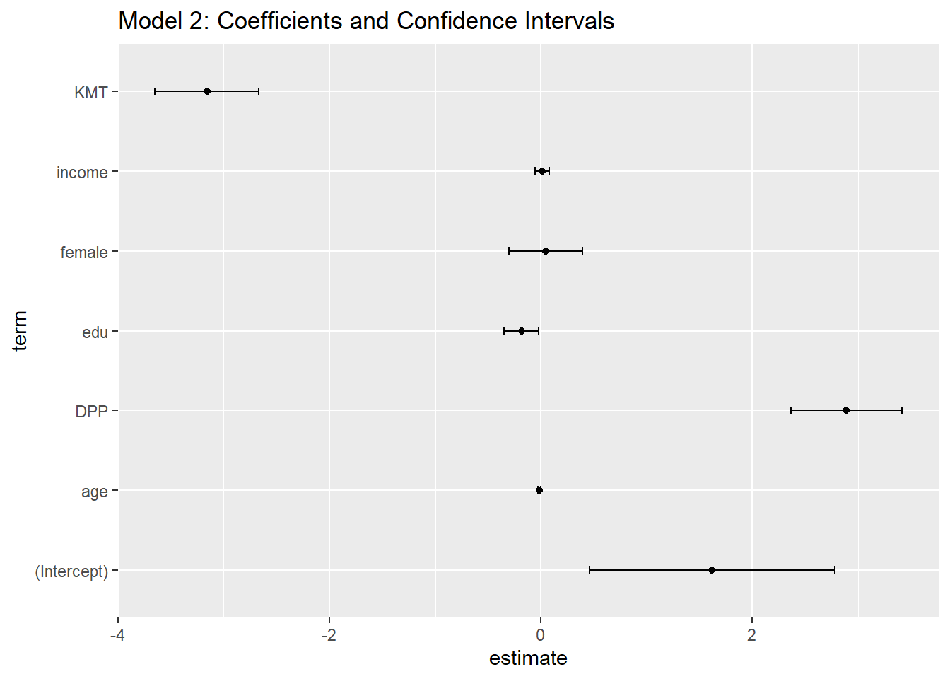
Interpretation for the updated model
Based on the output of the logistic regression model with additional predictors, here is the interpretation of the results:
Female: The coefficient for the female variable is 0.047406 with a p-value of 0.78930. The p-value is greater than 0.05, so the effect of the female variable is not statistically significant. This means that there is no evidence to suggest that female voters are more likely to vote for President Tsai compared to male voters, after controlling for other variables.
KMT: The coefficient for the KMT variable is -3.156273 with a p-value close to 0 (p < 2e-16). This indicates that respondents with a stronger KMT party affiliation are significantly less likely to vote for President Tsai.
DPP: The coefficient for the DPP variable is 2.888943 with a p-value close to 0 (p < 2e-16). This suggests that respondents with a stronger DPP party affiliation are significantly more likely to vote for President Tsai.
Age: The coefficient for the age variable is -0.011808 with a p-value of 0.09931. The p-value is slightly greater than 0.05, so the effect of age is not statistically significant at the 0.05 level. However, the negative coefficient suggests that older respondents are somewhat less likely to vote for President Tsai, but this relationship is weak.
Edu: The coefficient for the edu variable is -0.184604 with a p-value of 0.02632. The negative coefficient indicates that respondents with higher education levels are more likely to vote for President Tsai, and this effect is statistically significant (p < 0.05).
Income: The coefficient for the income variable is 0.013727 with a p-value of 0.68971. The p-value is greater than 0.05, so the effect of income is not statistically significant. This means that there is no evidence to suggest that income levels significantly influence the likelihood of voting for President Tsai.
In summary, the most significant predictors in this model are KMT and DPP party affiliations, which have strong and statistically significant effects on the likelihood of voting for President Tsai. Education also has a significant effect, while the female, age, and income variables are not statistically significant in this model.
Coefficient plots for the two models
Start:  AIC=793.13
votetsai ~ female + KMT + DPP + age + edu + income + Independence +
    Econ_worse + Govt_dont_care + Minnan_father + Mainland_father +
    Taiwanese

                  Df Deviance    AIC
- Govt_dont_care   1   767.14 791.14
- age              1   767.31 791.31
- female           1   767.40 791.40
- income           1   767.49 791.49
- Minnan_father    1   768.09 792.09
- edu              1   768.18 792.18
<none>                 767.13 793.13
- Econ_worse       1   769.82 793.82
- Mainland_father  1   774.99 798.99
- Independence     1   784.68 808.68
- Taiwanese        1   787.92 811.92
- DPP              1   884.02 908.02
- KMT              1   954.40 978.40

Step:  AIC=791.14
votetsai ~ female + KMT + DPP + age + edu + income + Independence +
    Econ_worse + Minnan_father + Mainland_father + Taiwanese

                  Df Deviance    AIC
- age              1   767.32 789.32
- female           1   767.40 789.40
- income           1   767.49 789.49
- Minnan_father    1   768.11 790.11
- edu              1   768.18 790.18
<none>                 767.14 791.14
- Econ_worse       1   769.84 791.84
+ Govt_dont_care   1   767.13 793.13
- Mainland_father  1   775.08 797.08
- Independence     1   784.68 806.68
- Taiwanese        1   787.92 809.92
- DPP              1   884.68 906.68
- KMT              1   954.41 976.41

Step:  AIC=789.32
votetsai ~ female + KMT + DPP + edu + income + Independence +
    Econ_worse + Minnan_father + Mainland_father + Taiwanese

                  Df Deviance    AIC
- female           1   767.59 787.59
- income           1   767.70 787.70
- Minnan_father    1   768.21 788.21
<none>                 767.32 789.32
- Econ_worse       1   770.11 790.11
- edu              1   770.33 790.33
+ age              1   767.14 791.14
+ Govt_dont_care   1   767.31 791.31
- Mainland_father  1   775.09 795.09
- Independence     1   784.72 804.72
- Taiwanese        1   787.93 807.93
- DPP              1   885.39 905.39
- KMT              1   954.61 974.61

Step:  AIC=787.59
votetsai ~ KMT + DPP + edu + income + Independence + Econ_worse +
    Minnan_father + Mainland_father + Taiwanese

                  Df Deviance    AIC
- income           1   767.95 785.95
- Minnan_father    1   768.49 786.49
<none>                 767.59 787.59
- edu              1   770.43 788.43
- Econ_worse       1   770.44 788.44
+ female           1   767.32 789.32
+ age              1   767.40 789.40
+ Govt_dont_care   1   767.58 789.58
- Mainland_father  1   775.21 793.21
- Independence     1   785.27 803.27
- Taiwanese        1   787.94 805.94
- DPP              1   886.58 904.58
- KMT              1   955.77 973.77

Step:  AIC=785.95
votetsai ~ KMT + DPP + edu + Independence + Econ_worse + Minnan_father +
    Mainland_father + Taiwanese

                  Df Deviance    AIC
- Minnan_father    1   768.87 784.87
<none>                 767.95 785.95
- edu              1   770.43 786.43
- Econ_worse       1   770.69 786.69
+ income           1   767.59 787.59
+ female           1   767.70 787.70
+ age              1   767.74 787.74
+ Govt_dont_care   1   767.95 787.95
- Mainland_father  1   775.59 791.59
- Independence     1   785.62 801.62
- Taiwanese        1   788.14 804.14
- DPP              1   888.19 904.19
- KMT              1   956.43 972.43

Step:  AIC=784.87
votetsai ~ KMT + DPP + edu + Independence + Econ_worse + Mainland_father +
    Taiwanese

                  Df Deviance    AIC
<none>                 768.87 784.87
- Econ_worse       1   771.48 785.48
- edu              1   771.59 785.59
+ Minnan_father    1   767.95 785.95
+ income           1   768.49 786.49
+ female           1   768.61 786.61
+ age              1   768.74 786.74
+ Govt_dont_care   1   768.86 786.86
- Mainland_father  1   775.96 789.96
- Independence     1   786.35 800.35
- Taiwanese        1   788.59 802.59
- DPP              1   888.66 902.66
- KMT              1   956.56 970.56
Call:
glm(formula = votetsai ~ KMT + DPP + edu + Independence + Econ_worse +
    Mainland_father + Taiwanese, family = binomial, data = TEDS_2016)

Deviance Residuals:
    Min       1Q   Median       3Q      Max
-3.0043  -0.3074   0.1731   0.4096   2.7622

Coefficients:
                Estimate Std. Error z value Pr(>|z|)
(Intercept)      0.05688    0.27971   0.203  0.83886
KMT             -2.88317    0.25561 -11.280  < 2e-16 ***
DPP              2.47837    0.27407   9.043  < 2e-16 ***
edu             -0.10296    0.06257  -1.645  0.09989 .
Independence     1.00339    0.24761   4.052 5.07e-05 ***
Econ_worse       0.30187    0.18640   1.619  0.10535
Mainland_father -0.85644    0.33052  -2.591  0.00956 **
Taiwanese        0.86729    0.19455   4.458 8.28e-06 ***
---
Signif. codes:  0 '***' 0.001 '**' 0.01 '*' 0.05 '.' 0.1 ' ' 1

(Dispersion parameter for binomial family taken to be 1)

    Null deviance: 1661.76  on 1256  degrees of freedom
Residual deviance:  768.87  on 1249  degrees of freedom
  (433 observations deleted due to missingness)
AIC: 784.87

Number of Fisher Scoring iterations: 6
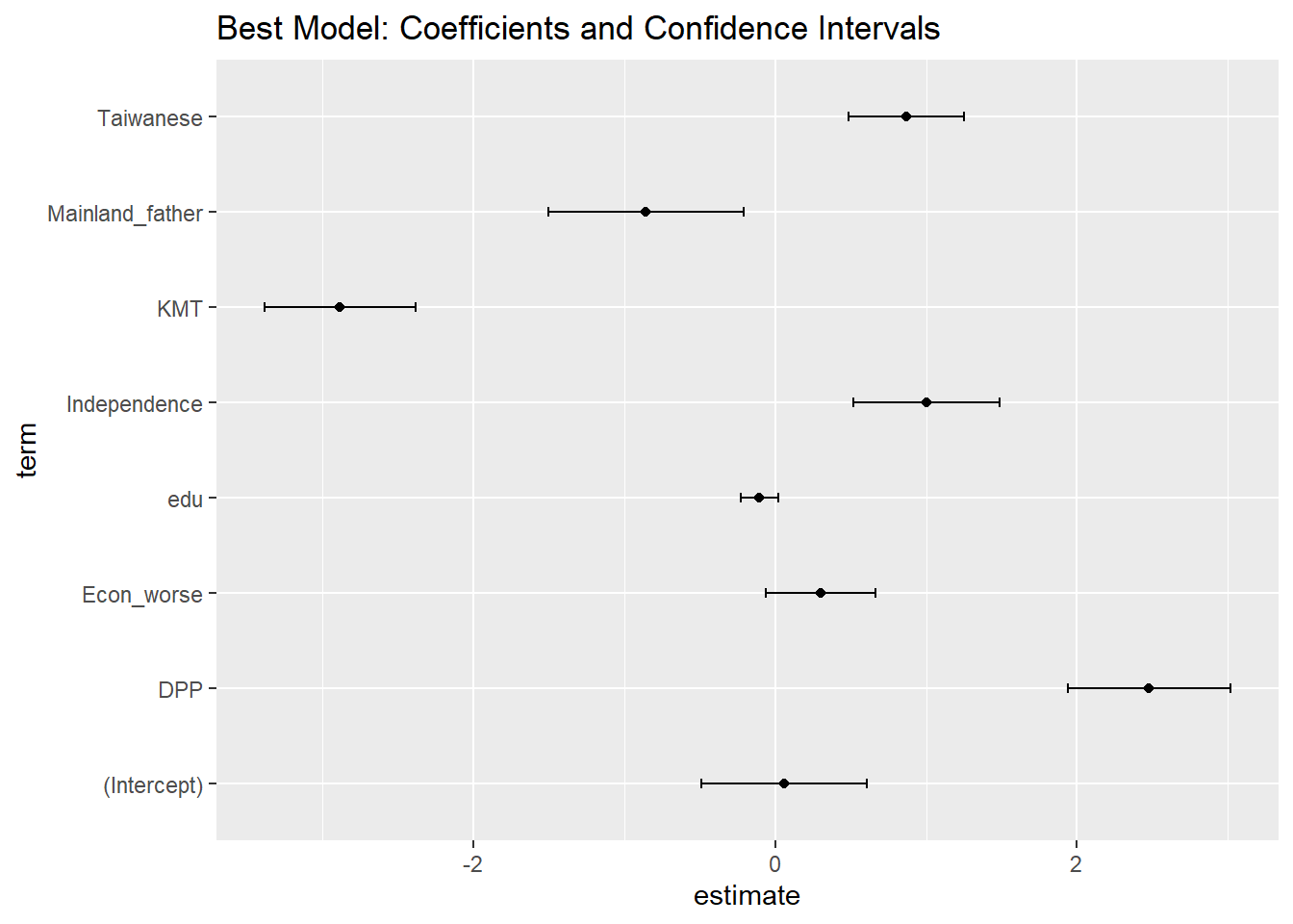
Interpreting the best model
This is the best model selected by stepAIC based on AIC criteria. The model predicts the likelihood of voting for Tsai Ing-wen (votetsai) using the following predictors: KMT, DPP, edu, Independence, Econ_worse, Mainland_father, and Taiwanese.
Here’s the interpretation of the model:
KMT (Kuomintang) Party ID: The coefficient is -2.88317, and it is highly significant (p < 2e-16). A one-unit increase in KMT affiliation is associated with a decrease in the log-odds of voting for Tsai Ing-wen by 2.88317 units, holding other variables constant. In other words, KMT supporters are less likely to vote for Tsai Ing-wen.
DPP (Democratic Progressive Party) Party ID: The coefficient is 2.47837, and it is highly significant (p < 2e-16). A one-unit increase in DPP affiliation is associated with an increase in the log-odds of voting for Tsai Ing-wen by 2.47837 units, holding other variables constant. DPP supporters are more likely to vote for Tsai Ing-wen.
Education (edu): The coefficient is -0.10296, and it is marginally significant (p = 0.09989). A one-unit increase in education level is associated with a decrease in the log-odds of voting for Tsai Ing-wen by 0.10296 units, holding other variables constant. More educated individuals are slightly less likely to vote for Tsai Ing-wen.
Independence: The coefficient is 1.00339, and it is highly significant (p = 5.07e-05). A one-unit increase in support for Taiwan’s independence is associated with an increase in the log-odds of voting for Tsai Ing-wen by 1.00339 units, holding other variables constant. Those who support Taiwan’s independence are more likely to vote for Tsai Ing-wen.
Economic evaluation (Econ_worse): The coefficient is 0.30187, and it is not significant (p = 0.10535). A one-unit increase in negative economic evaluation is associated with an increase in the log-odds of voting for Tsai Ing-wen by 0.30187 units, holding other variables constant. However, this effect is not statistically significant.
Mainland father (Mainland_father): The coefficient is -0.85644, and it is significant (p = 0.00956). A one-unit increase in being a descendent of mainland China is associated with a decrease in the log-odds of voting for Tsai Ing-wen by 0.85644 units, holding other variables constant. Individuals with mainland Chinese ancestry are less likely to vote for Tsai Ing-wen.
Self-identified Taiwanese (Taiwanese): The coefficient is 0.86729, and it is highly significant (p = 8.28e-06). A one-unit increase in self-identification as Taiwanese is associated with an increase in the log-odds of voting for Tsai Ing-wen by 0.86729 units, holding other variables constant. Self-identified Taiwanese are more likely to vote for Tsai Ing-wen.
The model has an AIC of 784.87, and the residual deviance is 768.87 on 1249 degrees of freedom. This model provides a better fit compared
Lab Assignment
 [1] "crim"    "zn"      "indus"   "chas"    "nox"     "rm"      "age"
 [8] "dis"     "rad"     "tax"     "ptratio" "black"   "lstat"   "medv"
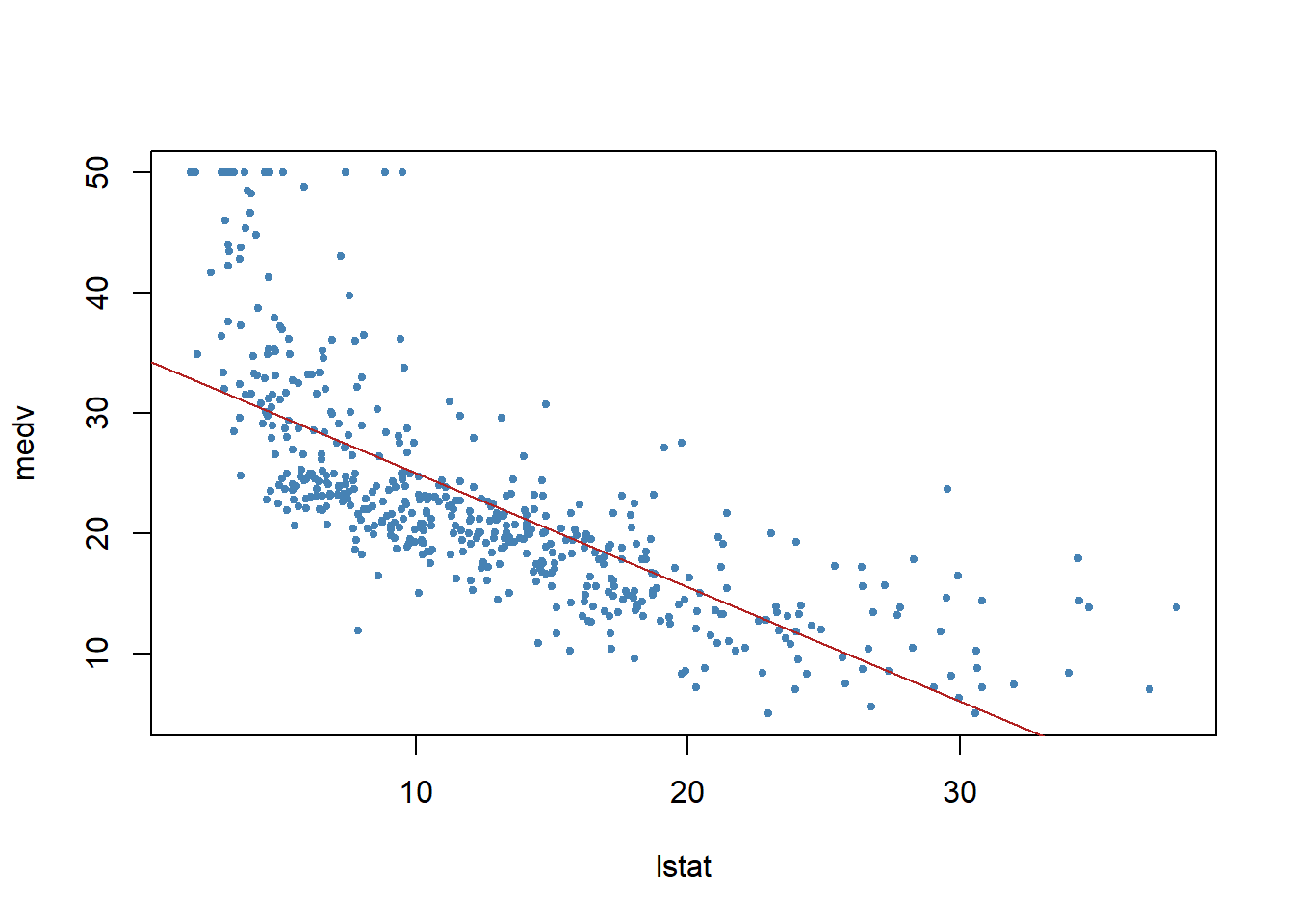
Call:
lm(formula = medv ~ lstat, data = Boston)

Coefficients:
(Intercept)        lstat
      34.55        -0.95
Call:
lm(formula = medv ~ lstat, data = Boston)

Residuals:
    Min      1Q  Median      3Q     Max
-15.168  -3.990  -1.318   2.034  24.500

Coefficients:
            Estimate Std. Error t value Pr(>|t|)
(Intercept) 34.55384    0.56263   61.41   <2e-16 ***
lstat       -0.95005    0.03873  -24.53   <2e-16 ***
---
Signif. codes:  0 '***' 0.001 '**' 0.01 '*' 0.05 '.' 0.1 ' ' 1

Residual standard error: 6.216 on 504 degrees of freedom
Multiple R-squared:  0.5441,    Adjusted R-squared:  0.5432
F-statistic: 601.6 on 1 and 504 DF,  p-value: < 2.2e-16
 [1] "coefficients"  "residuals"     "effects"       "rank"
 [5] "fitted.values" "assign"        "qr"            "df.residual"
 [9] "xlevels"       "call"          "terms"         "model"
                2.5 %     97.5 %
(Intercept) 33.448457 35.6592247
lstat       -1.026148 -0.8739505
       fit      lwr      upr
1 34.55384 33.44846 35.65922
2 29.80359 29.00741 30.59978
3 25.05335 24.47413 25.63256
4 20.30310 19.73159 20.87461
       fit       lwr      upr
1 34.55384 22.291923 46.81576
2 29.80359 17.565675 42.04151
3 25.05335 12.827626 37.27907
4 20.30310  8.077742 32.52846
Call:
lm(formula = medv ~ lstat + age, data = Boston)

Residuals:
    Min      1Q  Median      3Q     Max
-15.981  -3.978  -1.283   1.968  23.158

Coefficients:
            Estimate Std. Error t value Pr(>|t|)
(Intercept) 33.22276    0.73085  45.458  < 2e-16 ***
lstat       -1.03207    0.04819 -21.416  < 2e-16 ***
age          0.03454    0.01223   2.826  0.00491 **
---
Signif. codes:  0 '***' 0.001 '**' 0.01 '*' 0.05 '.' 0.1 ' ' 1

Residual standard error: 6.173 on 503 degrees of freedom
Multiple R-squared:  0.5513,    Adjusted R-squared:  0.5495
F-statistic:   309 on 2 and 503 DF,  p-value: < 2.2e-16
Call:
lm(formula = medv ~ ., data = Boston)

Residuals:
    Min      1Q  Median      3Q     Max
-15.595  -2.730  -0.518   1.777  26.199

Coefficients:
              Estimate Std. Error t value Pr(>|t|)
(Intercept)  3.646e+01  5.103e+00   7.144 3.28e-12 ***
crim        -1.080e-01  3.286e-02  -3.287 0.001087 **
zn           4.642e-02  1.373e-02   3.382 0.000778 ***
indus        2.056e-02  6.150e-02   0.334 0.738288
chas         2.687e+00  8.616e-01   3.118 0.001925 **
nox         -1.777e+01  3.820e+00  -4.651 4.25e-06 ***
rm           3.810e+00  4.179e-01   9.116  < 2e-16 ***
age          6.922e-04  1.321e-02   0.052 0.958229
dis         -1.476e+00  1.995e-01  -7.398 6.01e-13 ***
rad          3.060e-01  6.635e-02   4.613 5.07e-06 ***
tax         -1.233e-02  3.760e-03  -3.280 0.001112 **
ptratio     -9.527e-01  1.308e-01  -7.283 1.31e-12 ***
black        9.312e-03  2.686e-03   3.467 0.000573 ***
lstat       -5.248e-01  5.072e-02 -10.347  < 2e-16 ***
---
Signif. codes:  0 '***' 0.001 '**' 0.01 '*' 0.05 '.' 0.1 ' ' 1

Residual standard error: 4.745 on 492 degrees of freedom
Multiple R-squared:  0.7406,    Adjusted R-squared:  0.7338
F-statistic: 108.1 on 13 and 492 DF,  p-value: < 2.2e-16
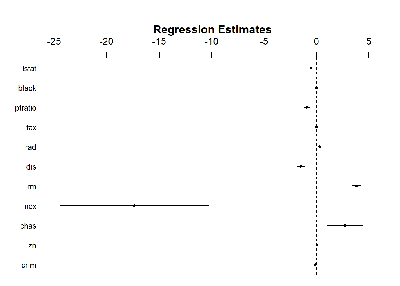
Call:
lm(formula = medv ~ crim + zn + chas + nox + rm + dis + rad +
    tax + ptratio + black + lstat, data = Boston)

Residuals:
     Min       1Q   Median       3Q      Max
-15.5984  -2.7386  -0.5046   1.7273  26.2373

Coefficients:
              Estimate Std. Error t value Pr(>|t|)
(Intercept)  36.341145   5.067492   7.171 2.73e-12 ***
crim         -0.108413   0.032779  -3.307 0.001010 **
zn            0.045845   0.013523   3.390 0.000754 ***
chas          2.718716   0.854240   3.183 0.001551 **
nox         -17.376023   3.535243  -4.915 1.21e-06 ***
rm            3.801579   0.406316   9.356  < 2e-16 ***
dis          -1.492711   0.185731  -8.037 6.84e-15 ***
rad           0.299608   0.063402   4.726 3.00e-06 ***
tax          -0.011778   0.003372  -3.493 0.000521 ***
ptratio      -0.946525   0.129066  -7.334 9.24e-13 ***
black         0.009291   0.002674   3.475 0.000557 ***
lstat        -0.522553   0.047424 -11.019  < 2e-16 ***
---
Signif. codes:  0 '***' 0.001 '**' 0.01 '*' 0.05 '.' 0.1 ' ' 1

Residual standard error: 4.736 on 494 degrees of freedom
Multiple R-squared:  0.7406,    Adjusted R-squared:  0.7348
F-statistic: 128.2 on 11 and 494 DF,  p-value: < 2.2e-16

Call:
lm(formula = medv ~ lstat * age, data = Boston)

Residuals:
    Min      1Q  Median      3Q     Max
-15.806  -4.045  -1.333   2.085  27.552

Coefficients:
              Estimate Std. Error t value Pr(>|t|)
(Intercept) 36.0885359  1.4698355  24.553  < 2e-16 ***
lstat       -1.3921168  0.1674555  -8.313 8.78e-16 ***
age         -0.0007209  0.0198792  -0.036   0.9711
lstat:age    0.0041560  0.0018518   2.244   0.0252 *
---
Signif. codes:  0 '***' 0.001 '**' 0.01 '*' 0.05 '.' 0.1 ' ' 1

Residual standard error: 6.149 on 502 degrees of freedom
Multiple R-squared:  0.5557,    Adjusted R-squared:  0.5531
F-statistic: 209.3 on 3 and 502 DF,  p-value: < 2.2e-16
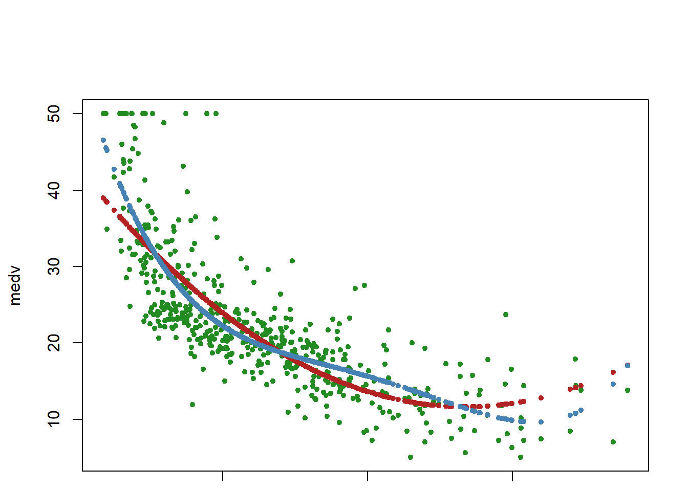
Call:
lm(formula = medv ~ lstat + I(lstat^2), data = Boston)

Residuals:
     Min       1Q   Median       3Q      Max
-15.2834  -3.8313  -0.5295   2.3095  25.4148

Coefficients:
             Estimate Std. Error t value Pr(>|t|)
(Intercept) 42.862007   0.872084   49.15   <2e-16 ***
lstat       -2.332821   0.123803  -18.84   <2e-16 ***
I(lstat^2)   0.043547   0.003745   11.63   <2e-16 ***
---
Signif. codes:  0 '***' 0.001 '**' 0.01 '*' 0.05 '.' 0.1 ' ' 1

Residual standard error: 5.524 on 503 degrees of freedom
Multiple R-squared:  0.6407,    Adjusted R-squared:  0.6393
F-statistic: 448.5 on 2 and 503 DF,  p-value: < 2.2e-16
 [1] "Sales"       "CompPrice"   "Income"      "Advertising" "Population"
 [6] "Price"       "ShelveLoc"   "Age"         "Education"   "Urban"
[11] "US"
     Sales          CompPrice       Income        Advertising
 Min.   : 0.000   Min.   : 77   Min.   : 21.00   Min.   : 0.000
 1st Qu.: 5.390   1st Qu.:115   1st Qu.: 42.75   1st Qu.: 0.000
 Median : 7.490   Median :125   Median : 69.00   Median : 5.000
 Mean   : 7.496   Mean   :125   Mean   : 68.66   Mean   : 6.635
 3rd Qu.: 9.320   3rd Qu.:135   3rd Qu.: 91.00   3rd Qu.:12.000
 Max.   :16.270   Max.   :175   Max.   :120.00   Max.   :29.000
   Population        Price        ShelveLoc        Age          Education
 Min.   : 10.0   Min.   : 24.0   Bad   : 96   Min.   :25.00   Min.   :10.0
 1st Qu.:139.0   1st Qu.:100.0   Good  : 85   1st Qu.:39.75   1st Qu.:12.0
 Median :272.0   Median :117.0   Medium:219   Median :54.50   Median :14.0
 Mean   :264.8   Mean   :115.8                Mean   :53.32   Mean   :13.9
 3rd Qu.:398.5   3rd Qu.:131.0                3rd Qu.:66.00   3rd Qu.:16.0
 Max.   :509.0   Max.   :191.0                Max.   :80.00   Max.   :18.0
 Urban       US
 No :118   No :142
 Yes:282   Yes:258
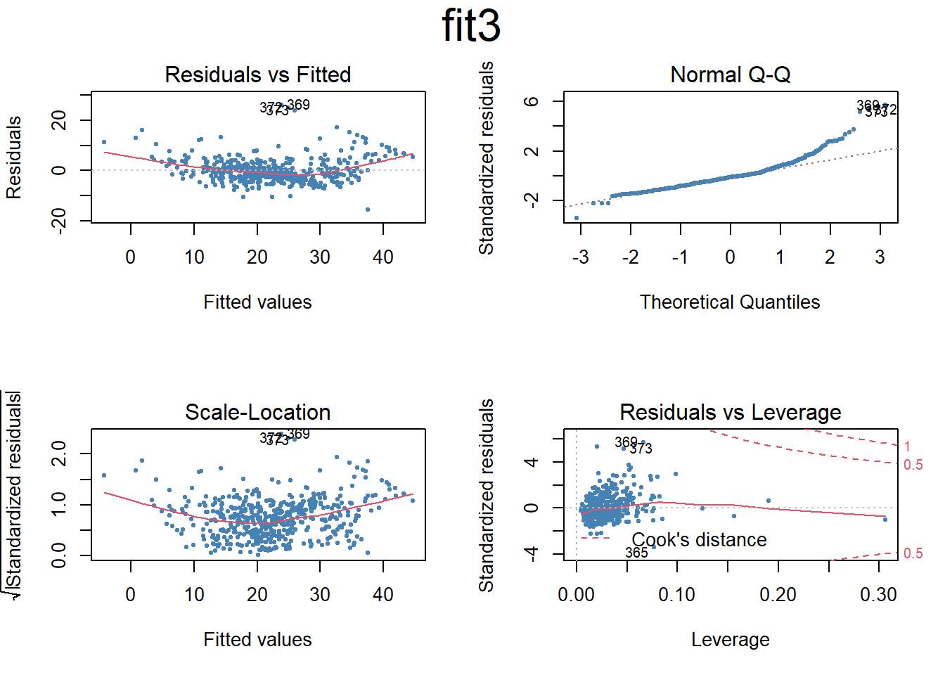
Call:
lm(formula = Sales ~ . + Income:Advertising + Age:Price, data = Carseats)

Residuals:
    Min      1Q  Median      3Q     Max
-2.9208 -0.7503  0.0177  0.6754  3.3413

Coefficients:
                     Estimate Std. Error t value Pr(>|t|)
(Intercept)         6.5755654  1.0087470   6.519 2.22e-10 ***
CompPrice           0.0929371  0.0041183  22.567  < 2e-16 ***
Income              0.0108940  0.0026044   4.183 3.57e-05 ***
Advertising         0.0702462  0.0226091   3.107 0.002030 **
Population          0.0001592  0.0003679   0.433 0.665330
Price              -0.1008064  0.0074399 -13.549  < 2e-16 ***
ShelveLocGood       4.8486762  0.1528378  31.724  < 2e-16 ***
ShelveLocMedium     1.9532620  0.1257682  15.531  < 2e-16 ***
Age                -0.0579466  0.0159506  -3.633 0.000318 ***
Education          -0.0208525  0.0196131  -1.063 0.288361
UrbanYes            0.1401597  0.1124019   1.247 0.213171
USYes              -0.1575571  0.1489234  -1.058 0.290729
Income:Advertising  0.0007510  0.0002784   2.698 0.007290 **
Price:Age           0.0001068  0.0001333   0.801 0.423812
---
Signif. codes:  0 '***' 0.001 '**' 0.01 '*' 0.05 '.' 0.1 ' ' 1

Residual standard error: 1.011 on 386 degrees of freedom
Multiple R-squared:  0.8761,    Adjusted R-squared:  0.8719
F-statistic:   210 on 13 and 386 DF,  p-value: < 2.2e-16
       Good Medium
Bad       0      0
Good      1      0
Medium    0      1